Time and Space Complexity
- 19 Jul, 2025
.jpg)
🧠 Classification of Data Structures
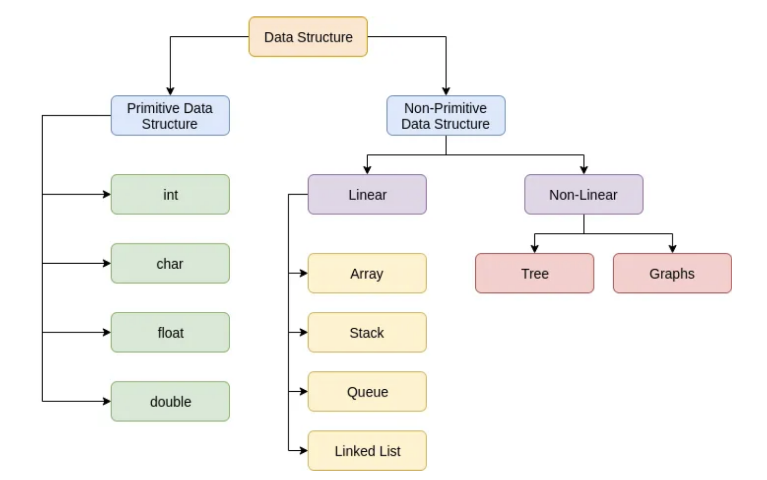
- Data Structures are categorized into Primitive and Non-Primitive types, where primitive types (like int, char, float, double) are the basic building blocks and are directly supported by most programming languages and hardware.
- Non-Primitive Data Structures are further divided into Linear and Non-Linear, where linear structures like Arrays, Stacks, Queues, and Linked Lists store elements sequentially — ideal for iteration, searching, or order-based operations.
- Non-Linear Structures like Trees and Graphs model complex relationships, like file systems, org charts, and web links.
- Understanding this hierarchy helps in pattern recognition during problem solving, e.g., a queue for BFS, a tree for recursion-heavy problems, and graphs for traversal/connectivity.
🧠 What is Time and Space Complexity?
1. Time Complexity (TC):
Time complexity measures how the number of operations grows with input size n.
Examples:
O(1): Constant timeO(n): LinearO(n^2): QuadraticO(log n): Logarithmic
✅ Focus on dominant term and worst-case complexity.
2. Space Complexity (SC):
Space complexity measures how much extra memory is used.
Examples:
- O(1): Constant extra space
- O(n): Hash map or array use
- O(n) call stack in recursion
📊 Time and Space Complexity Cheat Sheet
| Complexity | Name | Feasible Input Size (n) |
|---|---|---|
| O(1) | Constant | Instant |
| O(log n) | Logarithmic | Up to 10^18+ |
| O(n) | Linear | Up to 10^6–10^7 |
| O(n log n) | Linearithmic | Up to 10^5–10^6 |
| O(n^2) | Quadratic | Up to 10^3 |
| O(n^3) | Cubic | Up to 100 |
| O(2^n) | Exponential | Up to 20–25 |
| O(n!) | Factorial | Up to 10 |
🎯 How to Decide the Required TC/SC for an Interview Problem?
- n ≤ 10: Acceptable TC: O(n!), O(2^n) — use brute force or backtracking
- n ≤ 25: Acceptable TC: O(2^n) — bitmasking, subsets
- n ≤ 100: Acceptable TC: O(n^3) — triple nested loops
- n ≤ 1000: Acceptable TC: O(n^2) — dynamic programming
- n ≤ 1e5: Acceptable TC: O(n log n) or O(n) — sorting, sliding window
- n ≤ 1e6+: Acceptable TC: O(n), O(log n) — hashing, two pointers
📈 Big-O Complexity Chart
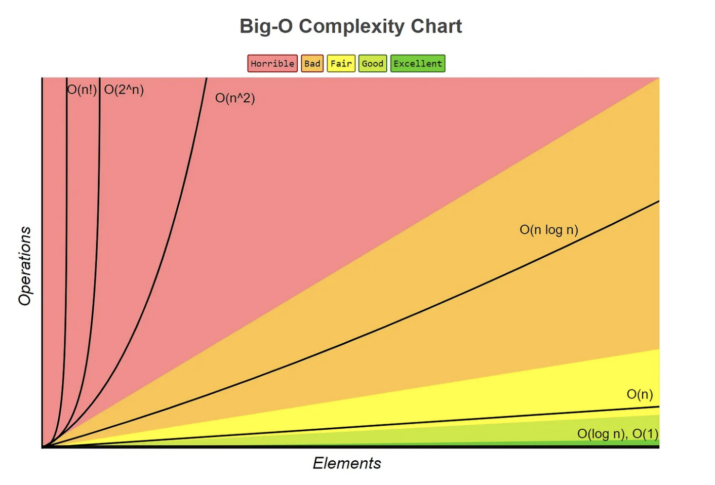
Color code:
- ✅ Excellent: O(1), O(log n)
- 🟡 Good to Fair: O(n), O(n log n)
- 🔴 Bad to Horrible: O(n^2), O(2^n), O(n!)
🌟 Highlights from the Article
- Big O notation (aka asymptotic analysis) measures how many operations an algorithm takes to complete — helping compare efficiency across solutions.
- ⚠️ There is no single fastest algorithm in all scenarios — performance varies depending on input state and best/worst-case paths.
📚 Want to go deeper?
Check out this excellent breakdown on Medium
Learning Big-O and complexity patterns early helps you write optimized code and choose the right approach in interviews.
✅ Practice Tip
Try analyzing the complexity of your solution before you code. Over time, this habit will lead to more efficient algorithms and better problem-solving instincts.